Time Series with Zillow’s Luminaire — Part I Data Exploration
Time Series with Zillow’s Luminaire — Part I Data Exploration

I sit at my local beach at midnight, enjoying the big moon casting sparkling lights on the ocean. The wavy moonlight path looks to me like a time series path, not always smooth but traceable. It shows me tranquility and serendipity.
I wrote a few articles on time series forecasting and anomaly detection. The Luminaire by the Zillow Tech Hub is the next one that I want to write an in-depth introduction. Are you doing time series forecasting and outlier detection now or in the near future? After reading this article, you will be running your time series model comfortably with Luminaire. Definitely read this article and the following series: Anomaly Detection for Time Series, Business Forecasting with Facebook’s “Prophet”, “A Technical Guide on RNN/LSTM/GRU for Stock Price Prediction”, and “Kalman Filter Explained!”.
Change Points Are Challenging in a Univariate Time Series
You typically deal with a daily, monthly, or quarterly time series (and high-frequency in IoT or stock tick data). If the number of data points is not enough to train a model, someone may suggest taking a longer time range. However, a longer time series also brings a new challenge because it contains more change points. A change point is the one that the data trend shifts abruptly. This happens in almost all time series such as finance, electricity consumption, manufacturing quality control, heart rate diagnostics, or human activity data. Let’s take the Dow Jones stock market daily data from 1970 to 2020 as an example. These years have so many macroeconomic events that have shifted the time series patterns from period to period. Human eyes may spot the change points easily, but an algorithm may not be able to. Since every time series has its own change points, it will be great to have a general algorithm to detect the change points automatically.
Time Series Data Preparation

The above flowchart is a typical data science process, each step involves sophisticated methods. The Luminaire module follows the procedure. The data preparation step includes exploratory data analysis, data cleaning, missing data imputation, and change point detection. The model specification step optimizes the best model specifications. The modeling step models the data for an appropriate model. These models include a structural model such as ARIMA or Decomposition, as well as a moving average or a Kalman Filter model. The forecasting considers how users need the forecasts such as real-time predictions, or streaming data anomaly detection.
Because each step involves considerable knowledge, I am going to walk you in three detailed articles. I have made the code in this article available for download via this github link.
The Luminaire by the Zillow Tech Hub
You may have seen the Zestimate in Zillow.com. The house price predictions are often so precise which become the essential references for home buyers. This is done by the Zillow Tech Hub.

The Luminaire, an open-source product, is another product that you will love to employ. You can visit the Luminaire Homepage Luminaire Github or this article Automatic and Self-aware Anomaly Detection at Zillow using Luminaire or this paper [1].
Luminaire is a python package that provides anomaly detection and forecasting functions that incorporate correlational and seasonal patterns as well as uncontrollable variations in the data over time.
How to Start
Luminaire currently requires Python 3.6 as described in the PyPI page.
I suggest you create a virtual environment for Python 3.6. Once you are
in the python 3.6 virtual environment, all you need to do is pip install Luminaire.
The Pruned Exact Linear Time (PELT) to Detect Change Points
An intuitive solution to detect change points is called Pruned Exact Linear Time (PELT) [2], [3]. I drew two graphs (A) and (B) to explain the method. The blue line is the time series. The horizontal orange line in the left graph (A) is the regression line. The distance from each point (shown as a white circle) to the regression line is represented by the vertical orange line. The regression line is determined by minimizing the sum of the distances to all the data points. Obviously the blue time series has two segments but (A) does not know.

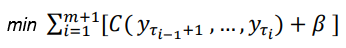
In contrast, the regression line in (B) is cut into two regression lines at the change point. The sum of the distances in (B) is much smaller than that in (A). By sliding the cut point from left to right of the time series, the algorithm can find the appropriate change point for the time series that minimizes the sum of the distances or errors. The equation below is the algorithm to search for the number of change points and the locations of change points. C(.) is the distance or the cost function. We also need to control for not creating too many line segments thus overfit the time series. So the term b (beta) is the number of segments as a penalty term to prevent the search yielding too many segments.
In the article “Finding the Change Points in a Time Series” I gave an in-depth review of change point detection that can be used for real-time applications. You can take a look.
(A) Let’s Start with the Minimum Data Exploration
I create a time series with two clusters. There is only one change point. Can Luminaire detect it?

The first step is to do exploratory data analysis (EDA). Luminaire’s DataExploration() lets you specify the attributes of the time series. The profile()
function executes the input instruction, imputes the missing data, and
detects change points. Here the time series is daily, so I specify
“freq=’D’”. The fill_rate is the minimum proportion of data availability in the recent data window, a fraction between 0 and 1. I just input 0.1.
There are two outputs of profile():
the first one is the interpolated data (I call it “ts2") and the second
one is the specification summary of this time series (I call it
“profile_summary”). The specification first says this operation is
successful (no failure). It implements the PELT algorithm and shows the
change point is [‘2018–07–04 00:00:00’]. Nice! The specification also
detects the start date and the end date of the time series. I asked it
to do a logarithmic transformation. So “is_log_transformed” shows False.
Nor do I input any minimum mean value for the time series, so
“min_ts_mean” shows None. These specifications will be tested later.
{'success': True, 'trend_change_list': ['2018-05-01 00:00:00', '2018-06-19 00:00:00', '2018-07-10 00:00:00', '2018-09-04 00:00:00', '2019-07-16 00:00:00'], 'change_point_list': ['2018-07-04 00:00:00'], 'is_log_transformed': False, 'min_ts_mean': None, 'ts_start': '2018-01-02 00:00:00', 'ts_end': '2020-12-31 00:00:00'}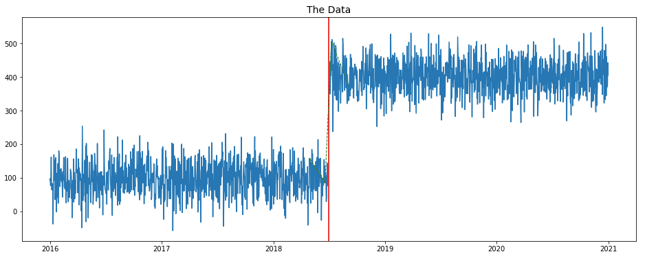
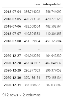
Do you notice I also saved the output in ts2? Luminaire imputes missing values by filling with the interpolated data. Since this time series has no missing, Luminaire just returns the same values.
(B) Data Exploration with a Stock Market Time Series
Let me use the stock market time series as a real example to explain the use of the data exploration specifications in Luminaire of this data exploration API reference.
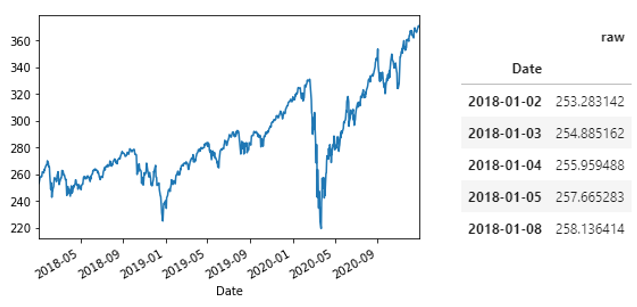
The first thing that we notice is the missing data have been imputed with interpolated values in the output of profile().
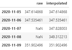
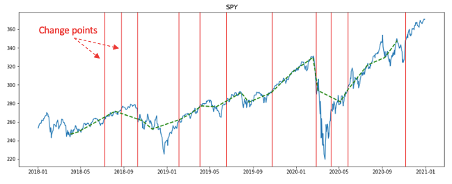
The data exploration step identifies the change points in a list. Luminaire also collects the trend change points in a list. The trend change points are where the trend changes from the previous data segment.
The input data: (755, 1)
The output data: (56, 2)
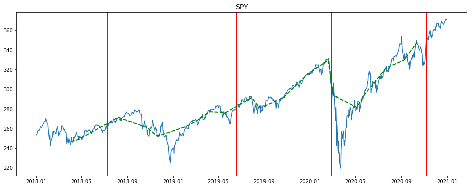
{'success': True, 'trend_change_list': ['2018-04-03 00:00:00', '2018-04-24 00:00:00', '2018-08-07 00:00:00', '2018-10-23 00:00:00', '2018-11-20 00:00:00', '2019-02-05 00:00:00', '2019-03-05 00:00:00', '2019-04-09 00:00:00', '2019-05-21 00:00:00', '2019-07-30 00:00:00', '2019-08-20 00:00:00', '2019-10-22 00:00:00', '2019-12-24 00:00:00', '2020-02-18 00:00:00', '2020-03-03 00:00:00', '2020-05-05 00:00:00', '2020-05-26 00:00:00', '2020-07-21 00:00:00', '2020-09-08 00:00:00', '2020-10-13 00:00:00'], 'change_point_list': ['2018-07-09 00:00:00', '2018-08-24 00:00:00', '2018-10-10 00:00:00', '2019-02-03 00:00:00', '2019-04-04 00:00:00', '2019-06-18 00:00:00', '2019-10-25 00:00:00', '2020-02-27 00:00:00', '2020-04-08 00:00:00', '2020-05-27 00:00:00', '2020-11-05 00:00:00'], 'is_log_transformed': None, 'min_ts_mean': None, 'ts_start': '2018-01-02 00:00:00', 'ts_end': '2020-12-30 00:00:00'}Below I plot the time series with the change points in red vertical lines and the trend segments in green dashed lines.
(C) Data Exploration: Logarithmic Transformation
You can test all the available parameters of this data exploration API reference. Below I illustrate one more specification: the logarithmic transformation. You just need to add one parameter “is_log_transformed=True”:
Luminaire does its data operation in the logarithmic scale as shown below.

Conclusion
Great job if you have made it this far! I have made the code in this article available for download via this github link. If you like to have a comprehensive review to advance in this topic, I suggest the following sequence:
- Part 1: “Anomaly Detection for Time Series“
- Part 2: “Detecting the Change Points in a Time Series”
- Part 3: “Algorithmic Trading with Technical Indicators in R”
- Part 4:“Kalman Filter Explained!”
- Part 5:“Business Forecasting with Facebook’s “Prophet”
- Part 6:“Time Series with Zillow’s Luminaire — Part I Data Exploration”
- Part 7:“Time Series with Zillow’s Luminaire — Part II Optimal Specifications”
- Part 8: “Time Series with Zillow’s Luminaire — Part III Modeling”
- Part 9:“A Technical Guide on RNN/LSTM/GRU for Stock Price Prediction”
Kindle and Paper Edition
The entire series on “explainable A.I.” is available in kindle or paper edition. Readers who prefer a kindle or a paper book can click here to find out more.

Citation
[1] Chakraborty, S., Shah, S., Soltani, K., Swigart, A., Yang, L., & Buckingham, K. (2020). Building an Automated and Self-Aware Anomaly Detection System. arXiv preprint arXiv:2011.05047. (arxiv_link)
[2] Killick Rebecca, Fearnhead P, Eckley Idris A(2012). Optimal detection of change points with a linear computational costs. JASA, 107, 1590–1598 (arxiv_link)
[3]
Gachomo Dorcas Wambui, Gichuhi Anthony Waititu, Jomo Kenyatta (2015).
The Power of the Pruned Exact Linear Time(PELT) Test in Multiple
Changepoint Detection American Journal of Theoretical and Applied
Statistics
Volume 4, Issue 6, November 2015, Pages: 581–586 (arxiv_link)
Data Science, Machine Learning, Artificial Intelligence

Share your ideas with millions of readers.


Comments
Post a Comment